Reestruturação e Junção de Dados

Treinamento em R

Introduction

The Challenge

Your director walks in:

“We need to identify the top 5 firms with the largest VAT gaps in the retail sector. Break them down by firm size—small, medium, and large—based on annual taxable income from CIT data. Can you have this ready by tomorrow?”

🤔 You think:

VAT gap = Expected VAT minus Actual VAT paid
I have quarterly VAT data in separate columns
Taxable income comes from CIT declarations (different file)
Firm characteristics (industry) are in yet another file
I need to join all three datasets together!

This module teaches you exactly how to solve this problem.

Today’s Roadmap

Understand tidy data principles
Reshape data between wide and long formats
Join multiple datasets together
Validate that your merges worked correctly
Build a complete analysis-ready dataset

Solving the Challenge: The Approach

What data do we have?

Quarterly VAT declarations (wide format: Q1, Q2, Q3, Q4 columns)
Annual CIT declarations (contains taxable income)
Firm registry (industry, firm characteristics)

What do we need to do?

Reshape: Convert quarterly VAT from wide to long format
Calculate: Annual VAT totals per firm
Join: Combine VAT with CIT to get taxable income
Categorize: Define firm size based on taxable income brackets
Join: Add firm characteristics (industry)
Filter & Rank: Select retail sector, find top 5 by size category

Key question: How do we get from messy, separate datasets to one clean analysis table?

Answer: By mastering reshaping and joins!

Tidy Data

Tidy Tax Administrative Data

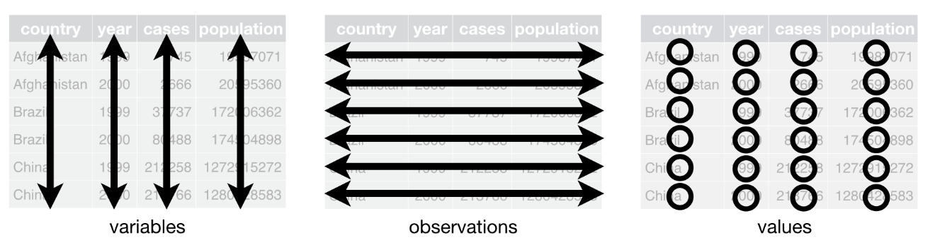
What is Tidy Data?

Tidy data organizes tax administrative data into a consistent, analysis-ready format:

Each variable is a column; each column is a variable.

Each observation is a row; each row is an observation.

Each value is a cell; each cell is a single value.

Let’s Look at This Dataset

Taxpayer ID	Tax Type	2021 Q1	2021 Q2	2021 Q3	2021 Q4
101	Income Tax	500	600	450	700
102	VAT	300	400	350	500

What’s the problem with this dataset?

Problems:

Quarter information (Q1, Q2, Q3, Q4) is spread across column names, not stored as data
Each row contains multiple observations (4 quarters worth of data)
Hard to filter for specific quarters or plot trends over time

What are the variables?

Taxpayer ID, Tax Type, Quarter, Payment Amount.

What constitutes a single observation in this dataset?

One observation is a specific tax payment for a taxpayer during a particular quarter.

Making It Tidy

How would you reshape the dataset to meet the three tidy characteristics?

Each variable is a column; each column is a variable.
Each observation is a row; each row is an observation.
Each value is a cell; each cell is a single value.

Tidy Version

Taxpayer ID	Tax Type	Quarter	Payment Amount
101	Income Tax	2021 Q1	500
101	Income Tax	2021 Q2	600
101	Income Tax	2021 Q3	450
101	Income Tax	2021 Q4	700
102	VAT	2021 Q1	300
102	VAT	2021 Q2	400
102	VAT	2021 Q3	350
102	VAT	2021 Q4	500

Why Does This Matter?

Tidy data makes analysis easier:

Calculate statistics by group (e.g., average payment by quarter)
Create visualizations with ggplot2
Apply functions consistently across observations
Join datasets without confusion

The Goal

Most of our work involves transforming messy data into tidy data, then analyzing it.

Part 1: Understanding Data Structure

Unit of Observation vs. Unit of Analysis

Unit of Observation
What each row represents in your raw data

Firm-quarter VAT filing
Firm-year CIT declaration
Individual transaction

Unit of Analysis
What you need for your analysis

Firm-year compliance rate
Industry-level trends
Aggregate tax gap

Example: You have firm-quarter observations but need firm-year analysis

Observations: FIRM_001 has 4 rows (Q1, Q2, Q3, Q4 of 2023)
Analysis: You want 1 row per firm-year with annual total

Wide vs. Long Format

Wide Format

Each time period is a column

firm_id	Q1_vat	Q2_vat	Q3_vat	Q4_vat
FIRM_01	1000	1200	1100	1300
FIRM_02	800	900	950	1000

Good for:

Calculating period-over-period changes
Summary tables
Spreadsheet-style viewing

Long Format

Each observation is a row

firm_id	quarter	vat_amount
FIRM_01	Q1	1000
FIRM_01	Q2	1200
FIRM_01	Q3	1100
FIRM_01	Q4	1300
FIRM_02	Q1	800

Good for:

Time series plots
Group-by operations
Most statistical analyses

Part 2: Reshaping Data

Why Pivot Longer?

Most common transformation in tax data analysis

Wide quarterly VAT data:

firm_id	vat_q1	vat_q2	vat_q3	vat_q4
FIRM_01	5000	5200	4800	5500

↓ Transform to long ↓

firm_id	quarter	vat_amount
FIRM_01	Q1	5000
FIRM_01	Q2	5200
FIRM_01	Q3	4800
FIRM_01	Q4	5500

Why? Required for:

Plotting time trends with ggplot2
Calculating quarterly growth rates
Group-by operations (e.g., average by quarter)
Any analysis that treats time as a variable

`pivot_longer()` Syntax

# Transform wide to long format
data_long <- data_wide %>%
  pivot_longer(
    cols = c(vat_q1, vat_q2, vat_q3, vat_q4),  # Which columns to pivot
    names_to = "quarter",                        # New column for old column names
    values_to = "vat_amount"                     # New column for values
  )

Breaking it down:

cols: Columns to reshape (the ones with repeated measurements)
names_to: Name for the new column that will hold the old column names
values_to: Name for the new column that will hold the values

Think of it as “unpacking”

You’re taking columns (Q1, Q2, Q3, Q4) and unpacking them into rows, storing the column name (Q1) and its value (5000) separately.

Live Example: Pivot Longer

# Show the wide format first
head(vat_wide, 3)

# Transform to long format
vat_long <- vat_wide %>%
  pivot_longer(
    cols = c(vat_q1, vat_q2, vat_q3, vat_q4),
    names_to = "quarter", 
    values_to = "vat_amount"
  )

# Show the result
head(vat_long, 6)

# Check dimensions
cat("Wide format:", nrow(vat_wide), "rows\n")
cat("Long format:", nrow(vat_long), "rows (4x more!)\n")

🏋️‍♀️ Exercise 1: Pivot Longer Practice

Task: Reshape the provided wide CIT data to long format

Open exercise_04_01_template.R
Load the wide CIT data from data/Intermediate/cit_wide.csv
Use pivot_longer() to transform year columns to long format
Verify the result has 4x more rows

10:00

Why Pivot Wider?

Less common, but important for specific tasks

Long format data:

firm_id	year	tax_type	amount
FIRM_01	2023	VAT	20000
FIRM_01	2023	CIT	15000
FIRM_02	2023	VAT	18000
FIRM_02	2023	CIT	12000

↓ Transform to wide ↓

firm_id	year	VAT	CIT
FIRM_01	2023	20000	15000
FIRM_02	2023	18000	12000

Why? Useful for:

Creating summary tables
Calculating ratios (VAT/CIT)
Period-over-period comparisons
Side-by-side comparisons

`pivot_wider()` Syntax

# Transform long to wide format
data_wide <- data_long %>%
  pivot_wider(
    id_cols = c(firm_id, year),      # Columns that identify each row
    names_from = tax_type,            # Column with values for new column names
    values_from = amount              # Column with values to spread
  )

Breaking it down:

id_cols: Columns that uniquely identify each row in the result
names_from: Which column contains the values that will become new column names
values_from: Which column contains the values to fill the new columns

Watch out for duplicates!

If you have multiple rows with the same combination of id_cols and names_from, pivot_wider() will create a list-column. Always check your data first!

Live Example: Pivot Wider

# Create sample data with VAT and CIT
tax_long <- tibble(
  firm_id = rep(c("FIRM_01", "FIRM_02"), each = 2),
  year = rep(2023, 4),
  tax_type = rep(c("VAT", "CIT"), 2),
  amount = c(20000, 15000, 18000, 12000)
)

# Show long format
print(tax_long)

# Transform to wide format
tax_wide <- tax_long %>%
  pivot_wider(
    id_cols = c(firm_id, year),
    names_from = tax_type,
    values_from = amount
  )

# Show result
print(tax_wide)

# Now we can easily calculate the VAT/CIT ratio
tax_wide <- tax_wide %>%
  mutate(vat_cit_ratio = VAT / CIT)

print(tax_wide)

Part 3: Joining Data

Why Join Data?

In tax administration, data lives in separate systems:

VAT System

Quarterly declarations
Input/output VAT
Refunds

CIT System

Annual declarations
Taxable income
Tax paid

Firm Registry

Industry
Size
Region

The Goal

Combine these datasets to analyze firm behavior across multiple tax types and characteristics.

The Relational Data Model

Three separate tables linked by firm_id:

Table 1: VAT (panel_vat)

firm_id	quarter	vat_amount
FIRM_01	Q1	5000
FIRM_01	Q2	5200

Table 2: CIT (panel_cit)

firm_id	year	cit_amount
FIRM_01	2023	15000
FIRM_02	2023	12000

Table 3: Firms (dt_firms)

firm_id	industry	size
FIRM_01	Retail	Medium
FIRM_02	Services	Small

The key: firm_id appears in all three tables, allowing us to link them together.

Join Keys: How R Matches Rows

Join key = The column(s) used to match rows between tables

Table A (VAT)

firm_id	vat
FIRM_01	5000
FIRM_02	4500
FIRM_03	6000

Table B (Firms)

firm_id	industry
FIRM_01	Retail
FIRM_02	Services

= ?

R matches rows where firm_id is the same

FIRM_01 → Match ✓
FIRM_02 → Match ✓
FIRM_03 → No match ?

What happens with FIRM_03?

That depends on the join type!

Join Types

`left_join()`: The Workhorse

Most commonly used join (80% of real-world cases)

Keeps all rows from left table

Table A (left)

firm_id	vat
FIRM_01	5000
FIRM_02	4500
FIRM_03	6000

Table B (right)

firm_id	industry
FIRM_01	Retail
FIRM_02	Services

Result: left_join(A, B)

firm_id	vat	industry
FIRM_01	5000	Retail
FIRM_02	4500	Services
FIRM_03	6000	NA

Note: FIRM_03 kept, but industry is NA

Why it’s the default

Preserves your primary dataset (the left table). Perfect for enriching existing data with additional attributes.

`left_join()` in Action

# Create sample data
vat_data <- tibble(
  firm_id = c("FIRM_01", "FIRM_02", "FIRM_03"),
  quarter = c("Q1", "Q1", "Q1"),
  vat_amount = c(5000, 4500, 6000)
)

firm_data <- tibble(
  firm_id = c("FIRM_01", "FIRM_02"),
  industry = c("Retail", "Services"),
  size = c("Medium", "Small")
)

# Show original tables
cat("VAT data:\n")
print(vat_data)

cat("\nFirm data:\n")
print(firm_data)

# Perform left join
vat_enriched <- left_join(vat_data, firm_data, by = "firm_id")

cat("\nAfter left_join:\n")
print(vat_enriched)

# Check row counts
cat("\nRow count check:\n")
cat("VAT data:", nrow(vat_data), "rows\n")
cat("Result:", nrow(vat_enriched), "rows (same!)\n")

🏋️‍♀️ Exercise 2: Your First Join

Task: Join CIT data to firm characteristics

Open exercise_04_02_template.R
Load panel_cit.csv and dt_firms.csv
Use left_join() to add firm characteristics to CIT data
Verify the row count matches the CIT data

10:00

`inner_join()`: Only Matches

Keeps only rows that exist in BOTH tables

Table A

firm_id	vat
FIRM_01	5000
FIRM_02	4500
FIRM_03	6000

Table B

firm_id	industry
FIRM_01	Retail
FIRM_02	Services

Result: inner_join(A, B)

firm_id	vat	industry
FIRM_01	5000	Retail
FIRM_02	4500	Services

Note: FIRM_03 dropped (no match in Table B)

Use case: Finding firms that filed BOTH VAT and CIT

# Firms that filed both taxes
both_taxes <- inner_join(vat_summary, cit_summary, by = c("firm_id", "year"))

`full_join()`: Everything

Keeps ALL rows from BOTH tables

Table A

firm_id	vat
FIRM_01	5000
FIRM_02	4500

Table B

firm_id	cit
FIRM_02	12000
FIRM_03	15000

Result: full_join(A, B)

firm_id	vat	cit
FIRM_01	5000	NA
FIRM_02	4500	12000
FIRM_03	NA	15000

Note: All firms kept, with NAs where no match

Use case: Comprehensive registry showing filers and non-filers for both taxes

# Complete view of all firms across both tax systems
complete_registry <- full_join(vat_data, cit_data, by = c("firm_id", "year"))

`anti_join()`: The Detective Tool

Returns rows from left table that DON’T have a match in right table

Table A (VAT filers)

firm_id	vat
FIRM_01	5000
FIRM_02	4500
FIRM_03	6000

Table B (CIT filers)

firm_id	cit
FIRM_01	15000
FIRM_02	12000

Result: anti_join(A, B)

firm_id	vat
FIRM_03	6000

Note: Only FIRM_03 returned (filed VAT but not CIT)

Critical for diagnostics!

Use anti_join() to find:

Firms that filed VAT but not CIT
Records that failed to merge (data quality issues)
Missing values in lookup tables

Visual Comparison: All Four Join Types

Same Example Data, Different Join Types:

Table A (VAT)

firm_id	vat
FIRM_01	5000
FIRM_02	4500
FIRM_03	6000

Table B (CIT)

firm_id	cit
FIRM_01	15000
FIRM_02	12000
FIRM_04	18000

Visual Comparison: Results

left_join(A, B)

firm_id	vat	cit
FIRM_01	5000	15000
FIRM_02	4500	12000
FIRM_03	6000	NA

Rows: 3 (all from A)

inner_join(A, B)

firm_id	vat	cit
FIRM_01	5000	15000
FIRM_02	4500	12000

Rows: 2 (only matches)

full_join(A, B)

firm_id	vat	cit
FIRM_01	5000	15000
FIRM_02	4500	12000
FIRM_03	6000	NA
FIRM_04	NA	18000

Rows: 4 (all from both)

anti_join(A, B)

firm_id	vat
FIRM_03	6000

Rows: 1 (in A, not in B)

Join Best Practices

Multiple-Key Joins

Sometimes one key isn’t enough

Problem: Same firm appears in multiple years

VAT data (panel)

firm_id	year	quarter	vat
FIRM_01	2022	Q1	5000
FIRM_01	2023	Q1	5200

Firm characteristics (also panel)

firm_id	year	industry
FIRM_01	2022	Retail
FIRM_01	2023	Retail

If you join only by firm_id, you’ll get duplicate matches!

Solution: Use multiple keys

# Join by both firm_id AND year
vat_enriched <- left_join(
  panel_vat, 
  dt_firms, 
  by = c("firm_id", "year")
)

Different Column Names

Real data often has inconsistent naming

Table A uses ‘id’

id	vat
FIRM_01	5000

Table B uses ‘firm_id’

firm_id	industry
FIRM_01	Retail

Solution: Specify the mapping

# Map id in left table to firm_id in right table
result <- left_join(
  table_a, 
  table_b, 
  by = c("id" = "firm_id")
)

# Or rename first (often cleaner)
table_a <- table_a %>% rename(firm_id = id)
result <- left_join(table_a, table_b, by = "firm_id")

Part 4: Validating Joins

Why Validation Matters

⚠️ Horror Story

You run a join. Everything looks fine. You send results to your director.

😱 The next day:

“These numbers look wrong. Why do we have 50,000 firm-year observations when we only have 5,000 firms?”

What happened? Duplicate keys in the right table caused a row explosion.

Lesson: Trust, but verify. ALWAYS validate your joins.

Common Join Problems

Duplicate keys → Row explosion
- Right table has multiple rows per key
- Result: More rows than you started with
Missing keys → Unwanted NAs
- Keys don’t match between tables
- Result: Lots of missing values
Data type mismatches → Zero matches
- One table has numeric IDs, the other has character IDs
- Result: No rows match at all
Typos in join column names
- You wrote by = "firm_id" but one table uses "firm_ID"
- Result: Error or cartesian join

Diagnostic Checklist

BEFORE joining:

# 1. Check for duplicate keys in both tables
panel_vat %>% 
  count(firm_id, year) %>% 
  filter(n > 1)

dt_firms %>% 
  count(firm_id, year) %>% 
  filter(n > 1)

# 2. Verify key columns exist and have same type
str(panel_vat$firm_id)
str(dt_firms$firm_id)

# 3. Check for missing values in key columns
sum(is.na(panel_vat$firm_id))
sum(is.na(dt_firms$firm_id))

Diagnostic Checklist (cont.)

AFTER joining:

# 4. Check row count - does it make sense?
cat("Before join:", nrow(panel_vat), "rows\n")
cat("After join:", nrow(merged_data), "rows\n")

# For left_join, should match left table (unless right has duplicates)
# For inner_join, should be less than or equal to either table

# 5. Find non-matches using anti_join
unmatched <- anti_join(panel_vat, dt_firms, by = c("firm_id", "year"))
cat("Unmatched rows:", nrow(unmatched), "\n")

# 6. Check for unexpected NAs in joined columns
merged_data %>%
  summarize(
    na_industry = sum(is.na(industry)),
    na_size = sum(is.na(size))
  )

# 7. Spot check a few rows
merged_data %>% 
  filter(firm_id == "FIRM_001") %>%
  select(firm_id, year, vat_amount, industry, size)

🏋️‍♀️ Exercise 3: Diagnose and Fix

Task: The provided join produces the wrong number of rows. Find and fix the problem.

Open exercise_04_03_template.R
Run the broken join code
Use diagnostic tools to identify the problem
Fix the join and validate the result

15:00

Part 5: Complete Workflow

Bringing It All Together

Realistic Scenario: Computing VAT Gap by Firm Size

Your director wants to identify top 5 firms with largest VAT gaps in retail, segmented by size.

The Pipeline:

Reshape: Convert quarterly VAT data from wide to long format
Aggregate: Calculate annual VAT totals per firm
Aggregate: Calculate annual taxable income from CIT data
Join: Combine VAT with CIT data to get taxable income
Join: Add firm characteristics (industry)
Categorize: Create firm size categories based on taxable income
- Small: Taxable Income < $50K
- Medium: $50K ≤ Taxable Income < $125K
- Large: Taxable Income ≥ $125K
Calculate: VAT gap = Expected VAT - Actual VAT paid
Filter & Rank: Select retail industry, find top 5 by size category
Validate: Check results make sense

Live Coding: Complete Pipeline

# Step 1: Reshape VAT from wide to long (if needed)
# In this example, panel_vat is already long, so we'll aggregate directly

# Step 2: Aggregate VAT to firm-year level
vat_annual <- panel_vat %>%
  mutate(year = lubridate::year(declaration_date)) %>%
  group_by(firm_id, year) %>%
  summarize(
    actual_vat = sum(vat_outputs - vat_inputs, na.rm = TRUE),
    vat_inputs = sum(vat_inputs, na.rm = TRUE),
    vat_outputs = sum(vat_outputs, na.rm = TRUE),
    quarters_filed = n(),
    .groups = "drop"
  )

# Step 3: Aggregate CIT to get taxable income
cit_annual <- panel_cit %>%
  mutate(year = lubridate::year(declaration_date)) %>%
  group_by(firm_id, year) %>%
  summarize(
    taxable_income = sum(taxable_income, na.rm = TRUE),
    .groups = "drop"
  )

# Step 4: Join VAT with CIT data
vat_cit <- left_join(
  vat_annual,
  cit_annual,
  by = c("firm_id", "year")
)

# Step 5: Join to firm characteristics
vat_with_firms <- left_join(
  vat_cit,
  dt_firms,
  by = c("firm_id", "year")
)

# Step 6: Create size categories based on taxable income
vat_with_firms <- vat_with_firms %>%
  mutate(
    firm_size = case_when(
      taxable_income < 50000 ~ "Small",
      taxable_income >= 50000 & taxable_income < 125000 ~ "Medium",
      taxable_income >= 125000 ~ "Large",
      is.na(taxable_income) ~ "Unknown",
      TRUE ~ "Unknown"
    )
  )

# Step 7: Calculate VAT gap (simplified example)
# VAT gap = Expected VAT - Actual VAT
vat_analysis <- vat_with_firms %>%
  mutate(
    expected_vat = vat_outputs * 0.15,  # Assuming 15% VAT rate
    vat_gap = expected_vat - actual_vat
  )

# Step 8: Filter to retail and find top 5 by size
top_gaps <- vat_analysis %>%
  filter(industry == "Retail", !is.na(vat_gap)) %>%
  group_by(firm_size) %>%
  slice_max(order_by = vat_gap, n = 5) %>%
  ungroup()

# Step 9: Validate
cat("Analysis summary:\n")
cat("Total firms analyzed:", nrow(vat_analysis), "\n")
cat("Retail firms:", sum(vat_analysis$industry == "Retail", na.rm = TRUE), "\n")
cat("Top gaps by size:\n")
print(top_gaps %>% count(firm_size))

# Save results
fwrite(
  vat_analysis, 
  here("data", "final", "vat_gap_analysis.csv")
)

cat("\n✓ VAT gap analysis complete!\n")

🏋️‍♀️ FINAL EXERCISE: VAT Gap Analysis

Task: Identify top 5 retail firms with largest VAT gaps, by size category

Open exercise_04_final_template.R
Follow the scaffolded steps to:
- Reshape wide VAT data to long format
- Calculate annual VAT totals per firm
- Create size categories based on taxable income
- Join VAT data with firm characteristics
- Calculate VAT gap for each firm
- Filter to retail industry
- Find top 5 firms per size category
Save results to data/Final/vat_gap_analysis.csv

This analysis will help identify compliance risks by firm size!

20:00

Wrap-Up

Key Takeaways

Tidy data follows three principles
- Each variable is a column
- Each observation is a row
- Each value is a cell
Use pivot_longer() for most reshaping tasks
- Wide to long is the most common transformation
Use left_join() as your default join
- Preserves your primary dataset
- Most common in practice (80% of cases)
Always validate your joins before proceeding
- Check row counts
- Look for unexpected NAs
- Use anti_join() to find non-matches
Follow a diagnostic workflow:
- Check keys → Join → Verify → Analyze

Resources

📖 Further Reading

R4DS Chapter 6: Data tidying
https://r4ds.hadley.nz/data-tidy
R4DS Chapter 20: Joins
https://r4ds.hadley.nz/joins
dplyr cheatsheet: Join functions reference
tidyr cheatsheet: Pivot functions reference

Great Work!

🎂 You can now:

Understand and apply tidy data principles
Transform data between wide and long formats
Combine multiple datasets using joins
Validate your merges to catch problems
Build analysis-ready datasets

You’ve solved the challenge!

You now know how to: - Reshape quarterly data to annual - Join firm characteristics - Calculate metrics like VAT gap - Segment by categories (firm size, industry) - Rank and identify top performers/risks

Practice makes perfect

The best way to master joins is to practice with real data. Don’t hesitate to experiment with different join types and see what happens!

Reestruturação e Junção de Dados

Introduction

The Challenge

Today’s Roadmap

Solving the Challenge: The Approach

Tidy Data

Tidy Tax Administrative Data

Let’s Look at This Dataset

Making It Tidy

Tidy Version

Why Does This Matter?

Part 1: Understanding Data Structure

Unit of Observation vs. Unit of Analysis

Wide vs. Long Format

Wide Format

Long Format

Part 2: Reshaping Data

Why Pivot Longer?

pivot_longer() Syntax

Live Example: Pivot Longer

🏋️‍♀️ Exercise 1: Pivot Longer Practice

Why Pivot Wider?

pivot_wider() Syntax

Live Example: Pivot Wider

Part 3: Joining Data

Why Join Data?

The Relational Data Model

Join Keys: How R Matches Rows

Join Types

left_join(): The Workhorse

left_join() in Action

🏋️‍♀️ Exercise 2: Your First Join

inner_join(): Only Matches

full_join(): Everything

anti_join(): The Detective Tool

Visual Comparison: All Four Join Types

Visual Comparison: Results

Join Best Practices

Multiple-Key Joins

Different Column Names

Part 4: Validating Joins

Why Validation Matters

Common Join Problems

Diagnostic Checklist

Diagnostic Checklist (cont.)

🏋️‍♀️ Exercise 3: Diagnose and Fix

Part 5: Complete Workflow

Bringing It All Together

Live Coding: Complete Pipeline

🏋️‍♀️ FINAL EXERCISE: VAT Gap Analysis

Wrap-Up

Key Takeaways

Resources

Great Work!

`pivot_longer()` Syntax

`pivot_wider()` Syntax

`left_join()`: The Workhorse

`left_join()` in Action

`inner_join()`: Only Matches

`full_join()`: Everything

`anti_join()`: The Detective Tool